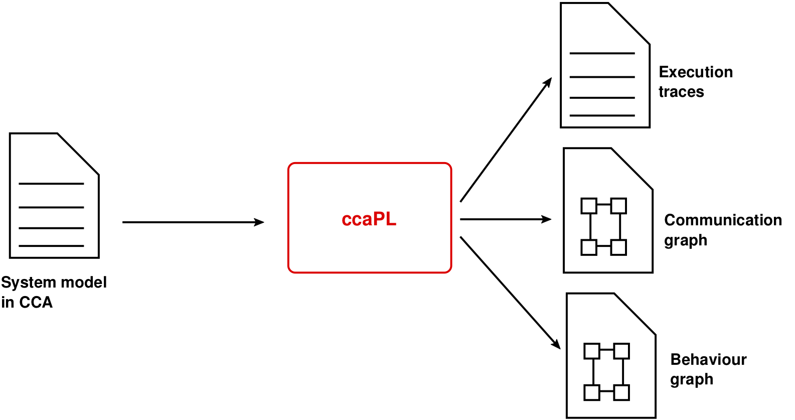
The Calculus of Context-aware Ambients (CCA) is a process calculus for modelling the behaviour of mobile and context-aware systems. The main features of the calculus include constructs for modelling mobility, context-awareness and concurrency which are important characteristics of pervasive/ubiquitous computing systems such as the Internet of Things (IoT) and smart systems. An ambient is an abstraction of a place where computation may happen. The single concept of ambient is used to model the behaviour of things, whether physical (e.g. devices) or virtual (e.g. software). An ambient can contain other ambients called child ambients, forming a hierarchical structure. This hierarchy of ambients is not fixed, but changes dynamically as mobile ambients move about; causing changes to the context of individual ambients. A context-aware ambient is able to sense changes to its context and adapt its behaviour automatically in response to those changes. Concurrent ambients run simultaneously and can communicate by message passing. CCA was inspired by the work by Luca Cardelli and Andrew D. Gordon on the Ambient Calculus.
CCA is developed and maintained by Francois Siewe. It is supported by software tools such as ccaPL, a simulation tool; and ccaSPIN, a model-checking tool. These have been applied to a variety of case studies; some of which can be found in Section 7.
The syntax of CCA is divided into 3 main syntactic categories: processes, denoted by P or Q; capabilities, denoted by M; and context-expressions, denoted by k. A context-expression is a condition over the context of the system; a capability denotes an atomic action; and a process describes a behaviour and is built from context-expressions and capabilities using specific operators as depicted below. Like in the π-calculus, the simplest entities in CCA are names, which are used to name things. We use lower-case letters n and x to denote names, some times with subscripts. We assume a countably-infinite set of names. Keywords are highlighted in red in the grammar.
| k ::= | true | holds for all context |
| 0 | holds for the empty context | |
| n=m | holds if the names n and m are lexically identical | |
| this | holds if the context is the current process | |
| not k | holds if k does not hold | |
| k |
holds if the context can be split into two parallel sub-contexts such that k1 holds for one and k2 holds for the other |
|
| k1 and k2 | holds if k1 holds and k2 holds | |
| k1 or k2 | holds if k1 holds or k2 holds | |
| n[k] | holds if the context is the ambient n and k holds for the internal context of the ambient n | |
| new(n, k) | holds if the context is of the form new n C and k holds for the context C. | |
| next k | holds if k holds for the internal context of some top-level ambient (aka spatial next modality) | |
| somewhere k | holds if k holds for the context or k holds for the internal context of some ambient (aka somewhere modality) |
The formal semantics of CEs is given in here.
| M ::= | skip | single transition step |
| in n | move in n | |
| out | move out | |
| del n | delete n | |
| α recv(y1, ..., yℓ) | input from location α and stored the received names in the variables y1, ..., yℓ | |
| α send(z1, ..., zℓ) | output the names z1, ..., zℓ to location α | |
| α x(z1, ..., zℓ) | call the process abstraction x defined in location α with actual parameters z1, ..., zℓ | |
| α ::= | @ | any parent |
| n@ | parent n | |
| # | any child | |
| n# | child n | |
| :: | any sibling | |
| n:: | sibling n | |
| ε | locally |
The capability skip always executes and terminates in a single transition step. The mobility capabilities in and out are defined as follows. An ambient that performs the capability in n moves into the sibling ambient n. The capability out moves the ambient that performs it out of that ambient's parent and into its parent's parent. The capability del n deletes an ambient of the form n[0]; i.e. an ambient n that has completed all its computations.
Ambients exchange messages using the output capability α send(z1, ..., zℓ) to send a list of names z1, ..., zℓ to a location α, and the input capability α recv(y1, ..., yℓ) to receive a list of names from a location α into the variables y1, ..., yℓ. The location α can be @ for any parent, n@ for a specific parent n, # for any child, n# for a specific child n, :: for any sibling, n:: for a specific sibling n, or ε (empty string) for the calling ambient itself.
A call to a process abstraction named x is done by a capability of the form α x(z1, ..., zℓ) where α specifies the location where the process abstraction is defined and z1, ..., zℓ are the actual parameters. A process call α x(z1, ..., zℓ) behaves like the process linked to x at the location α, in which each actual parameter zi, i = 1, . . ., ℓ is substituted for each occurrence of the corresponding formal parameter. A process call can only take place if the corresponding process abstraction is defined at the specified location. How to define a process abstraction is explained here.
The formal semantics of capabilities is given in here.
| P ::= | 0 | termination |
| M.P | sequential composition | |
| P | Q | parallel composition | |
| !P | replication | |
| new n P | name restriction | |
| n[P] | ambient | |
| {P} | brackets | |
| proc x(y1, ..., yℓ ) {P} | process abstraction definition | |
| let x1 = e1, ..., xℓ = eℓ in P | value assignment | |
| find y1, ..., yℓ : k for P | context-guarded name search | |
| <k>M.P | context-guarded prefix | |
| if <k1> M1.P1 ... <kℓ> Mℓ.Pℓ fi | context-guarded selection (if) | |
| if <k1> M1.P1 ... <kℓ> Mℓ.Pℓ else P fi | context-guarded selection (if-else) |
The process 0, aka inactivity process, does nothing and terminates immediately. The process P | Q denotes the concurrent execution of the process P and the process Q. The process new n P creates a new name n and the scope of that name is limited to the process P. The replication !P denotes a process which can always create a new copy of P, i.e. !P is equivalent to P | !P. Replication, first introduced in the π-calculus, can be used to implement both iteration and recursion. The process n[P] denotes an ambient named n whose behaviour is described by the process P. The process {P} behaves like P.
A process abstraction is a mechanism to give a name to a process and then use that name to call the process. A process abstraction definition has the form proc x(y1, ..., yℓ) {P}, where x is name given to the process P and the variables y1, ..., yℓ are the formal parameters. To call the process abstraction x, we write x(z1, ..., zℓ), where z1, ..., zℓ are the actual parameters. The process let x1 = e1, ..., xℓ = eℓ in P behaves like P{v1/x1, ..., vℓ/xℓ}, where vi is the value of the arithmetic expression ei, 1≤i≤ℓ. The process find y1, ..., yℓ : k for P searches for a list of names z1, ..., zℓ such that the environment satisfies the context expression k{z1/y1, ..., zℓ/yℓ} and then continues like P{z1/y1, ..., zℓ/yℓ}.
A context-guarded prefix <k>M.P is a process that waits until the environment satisfies the context expression k, then performs the capability M and continues like the process P. The dot symbol '.' denotes the sequential composition of processes. We let M.P denote the process <true>M.P , where true is a context expression satisfied by all context. A selection if <k1>M1.P1 ... <kℓ>Mℓ.Pℓ fi waits until at least one of the context-expressions (ki)1≤i≤ℓ holds say kj and the corresponding capability Mj can be executed; then proceeds non-deterministically like <kj>Mj.Pj. When the else part is specified like in if <k1>M1.P1 ... <kℓ>Mℓ.Pℓ else P fi, the process behaves like P if none of the ℓ branches can be taken.
In the graphical representation of ambients, the parallel composition operator "|" is optional and is understood as the sibling relationship between the ambients. For example, consider the following model of smarthome with one living room, one kitchen, one bathroom and two bedrooms. Suppose there is a television set in the living room, and Bob and Alice are in the kitchen while their son Peter is in his bedroom playing on his smartphone. This is specified by the following process.
smartHome[The graphical representation of this process is as follows.
In CCA, a process is described as a hierarchy of nested ambients. So, the context of each individual (sub-)process corresponds to the surrounding of that process in the hierarchy. This is obtained by replacing the process by a 'hole' in the hierarchy. A hole is represented by the symbol ⊙ and can be thought of as a place holder.
In CCA, a context is described by the following syntax, where the symbol C stands for context (environment), n ranges over names and P ranges over processes.
| C ::= | 0 | the empty context |
| ⊙ | the hole context | |
| P | ground context | |
| n[C] | ambient context | |
| C | P | parallel composition of context | |
| new n C | name restriction |
| C | 0 | = | C | |
| C1 | C2 | = | C2 | C1 | |
| C1 | (C2 | C3) | = | (C1 | C2) | C3 | |
| new n new m C | = | new m new n C | |
| new n C1 | C2 | = | new n (C1 | C2) | if n is not free in C2 |
| new n m[C] | = | m[new n C] | if n ≠ m |
| C1 = C2 | ⇒ | new n C1 = new n C2 | |
| C1 = C2 | ⇒ | C1 | C3 = C2 | C3 | |
| C1 = C2 | ⇒ | n[C1] = n[C2] |
The reflexive and transitive closure of this relation is denoted by ⇓* and is defined as:
C1 ⇓* C2 iff C1 = C2 or there exists a context C3 such that C1 ⇓ C3 and C3 ⇓* C2.
The context of the ambient bob in the smarthome system modelled the following. It is obtained by replacing the ambient bob in the system by the hole ⊙.
smartHome[The graphical representation of this context is as follows.
Similarly, the context of Peter's smartphone is the following:
smartHome[The graphical representation of this process is as follows.
| C | ⊨ | true | ||
| C | ⊨ | 0 | iff | C = 0 |
| C | ⊨ | n=n | ||
| C | ⊨ | this | iff | C = ⊙ |
| C | ⊨ | not k | iff | C ⊭ k |
| C | ⊨ | k1 | k2 | iff | there exist C1 and C2 such that C = C1 | C2 and C1 ⊨ k1 and C2 ⊨ k2 |
| C | ⊨ | k1 and k2 | iff | C ⊨ k1 and C ⊨ k2 |
| C | ⊨ | k1 or k2 | iff | C ⊨ k1 or C ⊨ k2 |
| C | ⊨ | n[k] | iff | there exists C' such that C = n[C'] and C' ⊨ k |
| C | ⊨ | new(n,k) | iff | there exists C' such that C = new n C' and C' ⊨ k |
| C | ⊨ | next k | iff | there exists C' such that C ⇓ C' and C' ⊨ k |
| C | ⊨ | somewhere k | iff | there exists C' such that C ⇓* C' and C' ⊨ k |
Following are examples of context-expressions that ambients can use to check their current situation.
| Name | Context-expression | Statement | |
|---|---|---|---|
| at(n) | = | somewhere(n[next(this | true)] | true) | My current location is the ambient n. |
| has(n) | = | somewhere(this | n[true] | true) | I am the current location of the ambient n. |
| with(n) | = | somewhere(next (this | true) | n[true] | true) | I am currently with the ambient n. |
| at(n, m) | = | somewhere(n[m[true] | true] | true) | The ambient m current location is the ambient n. |
| with(n, m) | = | somewhere(n[true] | m[true] | true) | The ambient n is currently with the ambient m. | empty(n) | = | somewhere(n[0] | true) | The ambient n is empty. |
Other context-expressions can be defined in a similar way.
An ambient can gather context information using the capability find described in Section 2.3. In the examples below, P denotes a process.
| Search process | Description |
|---|---|
| find n: at(n) for P | Find my current location. |
| find n: has(n) for P | Find a child ambient. |
| find n: with(n) for P | Find an ambient at my current location. |
| find n: at(n, m) for P | Find the current location of the ambient m. |
| find m: at(n, m) for P | Find an ambient that is at the location n. |
| find n, m: at(n, m) for P | Find an ambient and its location. |
| find m: with(n, m) for P | Find an ambient next to n. |
| find n, m: with(n, m) for P | Find two ambients who are at the same location. |
| find n: empty(n) for P | Find an empty ambient. |
| find n, m: at(n, m) and empty(m) for P | Find an empty ambient and its location. |
| (S1) | P | ≡ | P | (S13) | new n P | Q | ≡ | new n (P | Q), if n is not free in Q | |
| (S2) | P ≡ Q | ⇒ | Q ≡ P | (S14) | new n m[P] | ≡ | m[new n P], if n ≠ m | |
| (S3) | P ≡ Q, Q ≡ R | ⇒ | P ≡ R | (S15) | !P | ≡ | P | !P | |
| (S4) | P ≡ Q | ⇒ | new n P ≡ new n Q | (S16) | P | 0 | ≡ | P | |
| (S5) | P ≡ Q | ⇒ | P | R ≡ Q | R | (S17) | !0 | ≡ | 0 | |
| (S6) | P ≡ Q | ⇒ | !P ≡ !Q | (S18) | P.0 | ≡ | P | |
| (S7) | P ≡ Q | ⇒ | n[P] ≡ n[Q] | (S19) | new n 0 | ≡ | 0 | |
| (S8) | P ≡ Q | ⇒ | M.P ≡ M.Q | (S20) | <true> M.P | ≡ | M.P | |
| (S9) | P | Q | ≡ | Q | P | (S21) | P ≡ Q | ⇒ | <k>P ≡ <k>Q | |
| (S10) | P | (Q | R) | ≡ | (P | Q) | R | (S22) | (⊨ k1 ⇔ k2) | ⇒ | <k1>P ≡ <k2>P | |
| (S11) | new n new m P | ≡ | new m new n P | (S23) | P ≡ Q | ⇒ | proc x(y1, ..., yℓ) {P} ≡ proc x(y1, ..., yℓ) {Q} | |
| (S12) | {P} | ≡ | P | (S24) | C(let x1 = e1, ..., xℓ = eℓ in P) | ≡ | C(P{val(e1)/x1,..., val(eℓ)/xℓ}) |
| (R1) | proc x(y1,...,yℓ).{P} | x(z1,...,zℓ) → proc x(y1,...,yℓ).{P} | P{z1/y1,..., z1/yℓ} |
| (R2) | n[Q | proc x(y1,...,yℓ).{P}] | m[::x(z1,...,zℓ) | R] → n[Q | proc x(y1,...,yℓ).{P}] | m[P{z1/y1,..., z1/yℓ} | R] |
| (R3) | n[Q | proc x(y1,...,yℓ).{P}] | m[n::x(z1,...,zℓ) | R] → n[Q | proc x(y1,...,yℓ).{P}] | m[P{z1/y1,..., z1/yℓ} | R] |
| (R4) | proc x(y1,...,yℓ).{P} | m[@x(z1,...,zℓ) | R] → proc x(y1,...,yℓ).{P} | m[P{z1/y1,..., z1/yℓ} | R] |
| (R5) | n[proc x(y1,...,yℓ).{P} | m[n@x(z1,...,zℓ) | R]] → n[proc x(y1,...,yℓ).{P} | m[P{z1/y1,..., z1/yℓ} | R]] |
| (R6) | n[proc x(y1,...,yℓ).{P} | Q] | #x(z1,...,zℓ) → n[proc x(y1,...,yℓ).{P} | Q] | P{z1/y1,..., z1/yℓ} |
| (R7) | n[proc x(y1,...,yℓ).{P} | Q] | n#x(z1,...,zℓ) → n[proc x(y1,...,yℓ).{P} | Q] | P{z1/y1,..., z1/yℓ} |
| (R8) | recv(y1,...,yℓ).P | send(z1,...,zℓ).Q → P{z1/y1,..., z1/yℓ} | Q |
| (R9) | n[::recv(y1,...,yℓ).P | Q] | m[::send(z1,...,zℓ).R | S] → n[P{z1/y1,..., z1/yℓ} | Q] | m[R | S] |
| (R10) | n[::recv(y1,...,yℓ).P | Q] | m[n::send(z1,...,zℓ).R | S] → n[P{z1/y1,..., z1/yℓ} | Q] | m[R | S] |
| (R11) | n[m::recv(y1,...,yℓ).P | Q] | m[::send(z1,...,zℓ).R | S] → n[P{z1/y1,..., z1/yℓ} | Q] | m[R | S] |
| (R12) | n[m::recv(y1,...,yℓ).P | Q] | m[n::send(z1,...,zℓ).R | S] → n[P{z1/y1,..., z1/yℓ} | Q] | m[R | S] |
| (R13) | #recv(y1,...,yℓ).P | m[@send(z1,...,zℓ).Q | R] → P{z1/y1,..., z1/yℓ} | m[Q | R] |
| (R14) | m#recv(y1,...,yℓ).P | m[@send(z1,...,zℓ).Q | R] → P{z1/y1,..., z1/yℓ} | m[Q | R] |
| (R15) | #send(z1,...,zℓ).P | m[@recv(y1,...,yℓ).Q | R] → P | m[Q{z1/y1,..., z1/yℓ} | R] |
| (R16) | m#send(z1,...,zℓ).P | m[@recv(y1,...,yℓ).Q | R] → P | m[Q{z1/y1,..., z1/yℓ} | R] |
| (R17) | n[#recv(y1,...,yℓ).P | m[n@send(z1,...,zℓ).Q | R] | S] → n[P{z1/y1,..., z1/yℓ} | m[Q | R] | S] |
| (R18) | n[m#recv(y1,...,yℓ).P | m[n@send(z1,...,zℓ).Q | R] | S] → n[P{z1/y1,..., z1/yℓ} | m[Q | R] | S] |
| (R19) | n[#send(z1,...,zℓ).P | m[n@recv(y1,...,yℓ).Q | R] | S] → n[P | m[Q{z1/y1,..., z1/yℓ} | R] | S] |
| (R20) | n[m#send(z1,...,zℓ).P | m[n@recv(y1,...,yℓ).Q | R] | S] → n[P | m[Q{z1/y1,..., z1/yℓ} | R] | S] |
| (R21) | n[in m.P | Q] | m[R] → m[n[P | Q] | R] |
| (R22) | m[n[out.P | Q] | R] → n[P | Q] | m[R] |
| (R23) | C(M.P) → C'(Pσ) ⇒ C(<k>M.P) → C'(Pσ) if C ⊨ k |
| (R24) | C(find y1, ..., yℓ : k for P) → C(P{z1/y1,..., zℓ/yℓ}) if C ⊨ k{z1/y1,..., zℓ/yℓ} |
| (R25) | C(<ki>Mi.Pi) → C'(Piσ) ⇒ C(if <k1>M1.P1 ... <kℓ>Mℓ.Pℓ fi) → C'(Piσ) for some i, 1 ≤ i ≤ ℓ |
| (R26) | C(<ki>Mi.Pi) → C'(Piσ) ⇒ C(if <k1>M1.P1 ... <kℓ>Mℓ.Pℓ else P fi) → C'(Piσ) for some i, 1 ≤ i ≤ ℓ |
| (R27) | C(if <k1>M1.P1 ... <kℓ>Mℓ.Pℓ else P fi) → C(P) if ∀ i ∈ [1, ℓ] ∄ (C', σ) such that C(<ki>Mi.Pi) → C'(Piσ) |
| (R28) | skip.P → P |
| (R29) | del n.P | n[0] → P |
| (R30) | P → P' ⇒ new n P → new n P' |
| (R31) | P ≡ Q, Q → Q', Q' ≡ P' ⇒ P → P' |
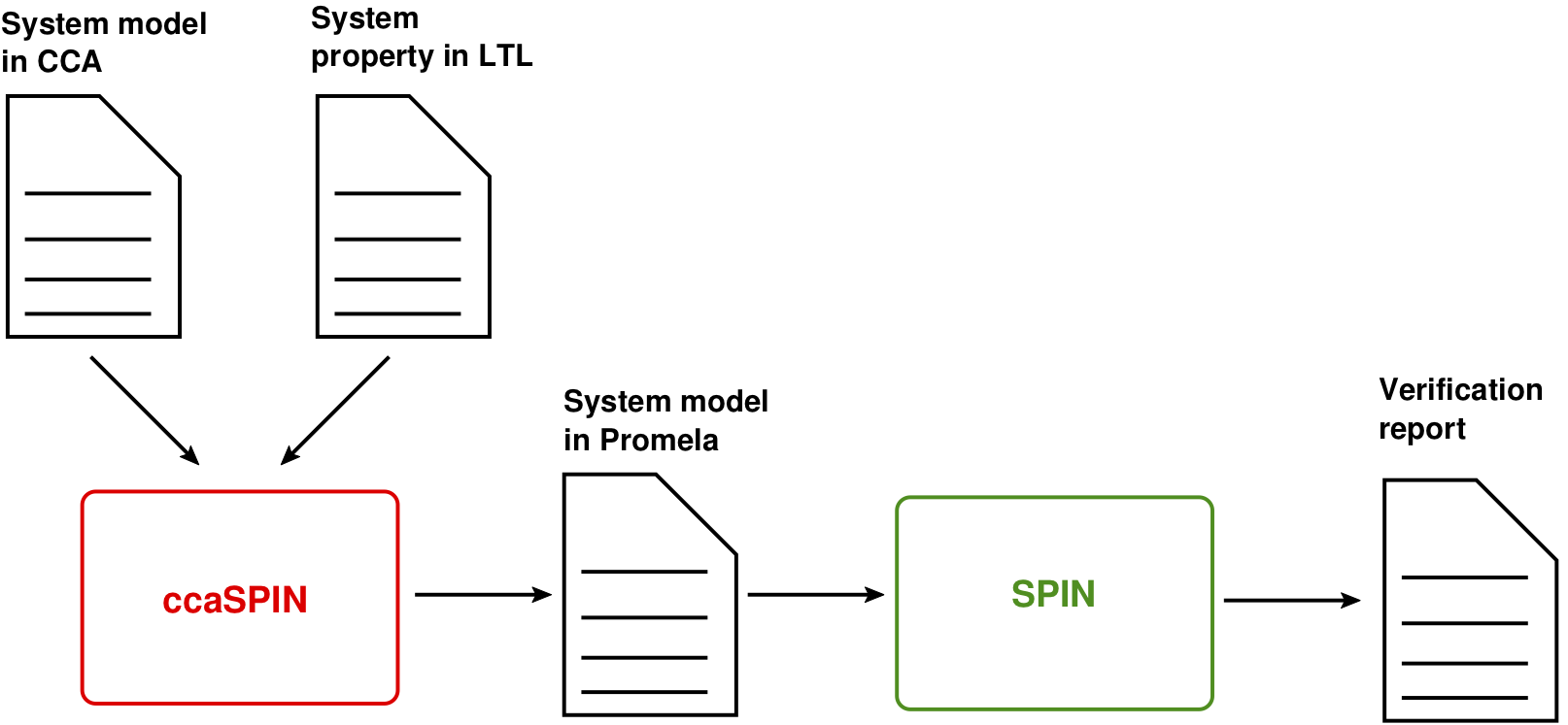
A CCA specification can be executed using the CCA interpreter ccaPL and automatically verified using the CCA model-checking tool ccaSPIN or the runtime verification tool ccaRV.
The textual format highlights the system's transitions relatively to the structural congruence relation (≡) and the reduction relation (→) defined in Section 3.3. A sample of the textual execution output is given in Fig. xx, where the symbol <--> represents the structural congruence relation and the symbol --> denotes the reduction relation. The meaning of each execution step (aka transition) is explained in a pair of curly brackets { ... }. The command line for generating a textual execution output is as follows:
java -jar ccaPL.jar -e myprog.cca
The graphical format depicts the interaction between the different ambients of the system in terms of the communication between them and their mobility. The communication graph is a sequence diagram that shows the message passing between the ambients. An example of communication graph is given in Fig. xx, where:
java -jar ccaPL.jar -g myprog.cca
The generated graph is stored in the file myprog.jpg.
The behaviour graph is similar to the communication graph, but also shows the ambient movements. An example is shown in Fig. xx, where a box labelled as X --> Y on the timeline of an ambient B indicates a transition in which the ambient B moves from a location X into a location Y. To create a behaviour graph, use the command line:
java -jar ccaPL.jar -gx myprog.cca
This will generate 2 graphs: a communication graph stored in the file myprog_0.jpg and the corresponding behaviour graph in the file myprog_1.jpg.
From version 5.06 you can generate the graphs in an image format other than jpg using the option -gXXX or -gxXXX, where XXX stands for the image format like ps, eps, pdf, gif, tif, png, vsg, json and so on.
NB: the generation of the graphical output requires that the Graphviz package be installed on your computer.
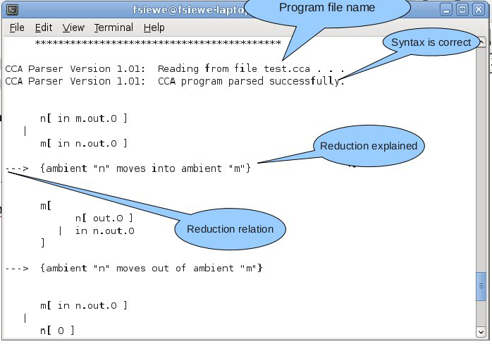
Fig. XX:
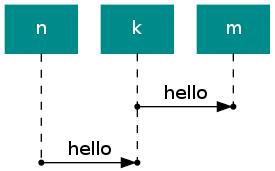
Fig. XX:
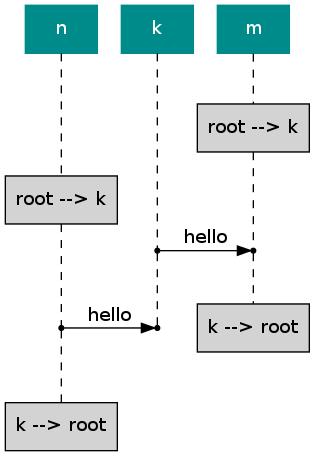
Fig. XX:
The declaration section begins with the keyword BEGIN_DECLS and ends with the keyword END_DECLS. There are 2 types of declarations:
A defintion of context-expression has the form: def f(x1, ..., xn) = { k } , where
Execution directives are used to control how processes are executed or to filter the execution output. Below is the list of the ccaPL execution directives.
To install ccaSPIN on your computer, download into your working directory the most recent version of ccaSPIN.jar below:
| f, g ::= | true | false | constants |
| p | a name | |
| a == b | a != b | boolean expressions where ... | |
| a < b | a <= b | a and b are names or ... | |
| a > b | a >= b | arithmetic expressions | |
| [] f | always f | the temporal operator always | |
| <> f | eventually f | the temporal operator eventually | |
| ! f | the boolean operator for negation | |
| f U g | f until g | the temporal operator strong until | |
| f W g | f weakuntil g | the temporal operator weak until | |
| f V g | f release g | the temporal operator release; the dual of U, i.e. !(!f U !g) | |
| f && g | f and g | the boolean operator for logical and | |
| f | | g | f or g | the boolean operator for logical or | |
| f -> g | f implies g | the boolean operator for logical implication | |
| f <-> g | f equivalent g | the boolean operator for logical equivalence | |
| a, b ::= | n | a name or an integer value |
| _nba | total number of ambients in the sysem | |
| _prt(a) | parent ambient of an ambient a | |
| _nbc(a) | number of child ambients of an ambient a | |
| aexp | arithmetic expression |
The meaning of the boolean operators is the as in the predicate logic. We summarise the semantics of the temporal operators as follows.
However, you can save the generated Promela program into a file say myprog.pml with the following command line.
The program file myprog.pml can then be analysed using SPIN. For more information about how to use the SPIN model-checker, visit the SPIN website here.